Reverse Engineering the HLTV 2.0 Rating

TL;DR:
0.0073*KAST + 0.3591*KPR + -0.5329*DPR + 0.2372*Impact + 0.0032*ADR + 0.1587 ≈ Rating 2.0
The longer tale:
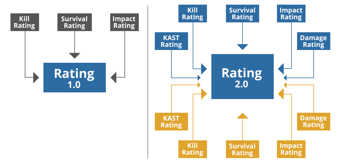
HLTV upgraded their ratings from 1.0 to 2.0 in the summer of 2017. Unlike the previous rating, HLTV decided to keep the formula of their 2.0 rating confidential. “The exact formula won’t be public this time” says their blog post. Yet, in the same blog post they list the 5 variables they use to calculate it.
I googled away, to see if someone had already reverse-engineered the formula - yet to my surprise I found little online. In fact, when googling I only found HLTV user-content asking about the formula. It almost feels as if there’s some mystery around the secret HLTV 2.0 rating formula.
After some thinking, I figured the formula must be a linear equation. So with enough data, I should be able to find a simple linear model which can estimate the coefficients of the variables. In other words, we know the variables they use, we’ll assume they just add them all together with a certain weight for each variable. They do say it’s calculated differently for CT and T side - but that complicates things, so let’s just ignore that for now.
First of all, we need some data to try and reverse the formula. I simply used an interactive scrapy shell to extract the links to each player profile from: https://www.hltv.org/stats/players. Once I had the links for the players, I simply built a small spider to crawl the following data from the players profiles: Player Name, Rating Version (some had their 1.0 rating), Rating, KAST, KPR, DPR, Impact, and ADR. That looks something like this:
import scrapy
import pandas as pd

links = pd.read_csv('player_links.csv')
links.columns = ['link']

links = list(links.link)

class HLTVSpider(scrapy.Spider):
    name = 'ratings'
    start_urls = links

    custom_settings = {
        'DOWNLOAD_DELAY': 1,
    }


    def parse(self, response):
        yield {
            'player': response.xpath('/html/body/div[2]/div/div[2]/div[1]/div[2]/div[6]/div[2]/div[1]/h1/text()').get(),
            'ratingVersion': response.xpath('/html/body/div[2]/div/div[2]/div[1]/div[2]/div[6]/div[2]/div[2]/div[1]/div[1]/text()').get(),
            'rating': response.xpath('/html/body/div[2]/div/div[2]/div[1]/div[2]/div[6]/div[2]/div[2]/div[1]/div[2]/div[1]/text()').get(),
            'kast': response.xpath('/html/body/div[2]/div/div[2]/div[1]/div[2]/div[6]/div[2]/div[2]/div[3]/div[2]/div[1]/text()').get(),
            'kpr': response.xpath('/html/body/div[2]/div/div[2]/div[1]/div[2]/div[6]/div[2]/div[3]/div[3]/div[2]/div[1]/text()').get(),
            'dpr': response.xpath('/html/body/div[2]/div/div[2]/div[1]/div[2]/div[6]/div[2]/div[2]/div[2]/div[2]/div[1]/text()').get(),
            'impact': response.xpath('/html/body/div[2]/div/div[2]/div[1]/div[2]/div[6]/div[2]/div[3]/div[1]/div[2]/div[1]/text()').get(),
            'adr': response.xpath('/html/body/div[2]/div/div[2]/div[1]/div[2]/div[6]/div[2]/div[3]/div[2]/div[2]/div[1]/text()').get(),
        }
Great - now we have some initial data to work with. First of all, let’s drop all players with 1.0 rating as we don’t care about that rating. The data needs some minor cleaning, but that’s done quickly. We just want all our data to be numbers - so we need to remove the % sign from KAST. I clean data in an interactive shell, so I don’t have the snippet. But something as simple as .rstrip(’%’) should do the job.
Sweet, we have clean data now. Let’s move on.
We’ve assumed a linear function, so let’s try to simply regress the data with a linear regression - the easiest and simplest way to approach this. While simple, linear regression will give us coefficients which are those weights we want to multiply our variables by before adding them together. In other words, it makes everything very interpretable. We can explore more complex models later on, if required.
import pandas as pd
from sklearn.model_selection import train_test_split
from sklearn.linear_model import LinearRegression
from sklearn.metrics import mean_absolute_error, r2_score, mean_squared_error

df = pd.read_csv('ratings2.csv')

y = df['rating']
X = df.drop(['rating', 'player', 'ratingVersion'], axis=1)

X_train, X_test, y_train, y_test = train_test_split(X, y, random_state=42,
                                                    test_size=0.2)

regr = LinearRegression()
regr.fit(X_train, y_train)

y_pred = regr.predict(X_test)

print(f'Coefficients: {regr.coef_}')

print(f'R2 score:{r2_score(y_test, y_pred)}')
print(f'RMSE:{mean_squared_error(y_test, y_pred, squared=False)}')
print(f'MAE:{mean_absolute_error(y_test, y_pred)}')

___________________________________________________________________________
OUTPUT

Coefficients: [ 0.00738764  0.35912389 -0.5329508   0.2372603   0.0032397 ]
Intercept: 0.15872723249055132
R2 score:0.9950978389640099
RMSE:0.004564354645876378
MAE:0.0020833333333333307
Hold up. That doesn’t look too bad. A couple of things that stand out to me are the 0.995 R2 score, that both error measures are smaller than 0.01, and that we have a negative coefficient? Let’s take a look further at what’s going on there.
The errors are interesting, because ratings only have 2 decimal places. So maybe if we round our predictions to 2 decimal places, we’ll get a better result? Oh - and I just checked the data and the third variable - which was given a negative coefficient - is deaths per round. That makes sense, the less you die the better your rating.
Let’s print some of the test data, to visually see our errors:
Actual: 1.1; Predicted: 1.1; Error: 0.0
Actual: 0.99; Predicted: 0.99; Error: 0.0
Actual: 1.04; Predicted: 1.04; Error: 0.0
Actual: 1.04; Predicted: 1.04; Error: 0.0
Actual: 1.13; Predicted: 1.13; Error: 0.0
Actual: 1.03; Predicted: 1.03; Error: 0.0
Actual: 1.07; Predicted: 1.07; Error: 0.0
Actual: 1.12; Predicted: 1.12; Error: 0.0
Actual: 1.15; Predicted: 1.15; Error: 0.0
Actual: 1.03; Predicted: 1.03; Error: 0.0
Actual: 1.12; Predicted: 1.12; Error: 0.0
Actual: 1.14; Predicted: 1.14; Error: 0.0
Actual: 1.01; Predicted: 1.01; Error: 0.0
Actual: 1.07; Predicted: 1.07; Error: 0.0
Actual: 1.04; Predicted: 1.05; Error: 0.010000000000000009
Actual: 0.93; Predicted: 0.92; Error: 0.010000000000000009
Actual: 1.21; Predicted: 1.21; Error: 0.0
Actual: 0.99; Predicted: 0.99; Error: 0.0
Actual: 1.04; Predicted: 1.04; Error: 0.0
Actual: 1.06; Predicted: 1.06; Error: 0.0
Actual: 1.1; Predicted: 1.1; Error: 0.0
Actual: 1.13; Predicted: 1.12; Error: 0.009999999999999787
Actual: 1.07; Predicted: 1.07; Error: 0.0
Actual: 1.02; Predicted: 1.02; Error: 0.0
Actual: 1.08; Predicted: 1.08; Error: 0.0
Actual: 1.19; Predicted: 1.19; Error: 0.0
That looks pretty good. We’re only ever wrong by 0.01 - but overall we calculate most of the ratings correctly. As we saw above, HLTV claims that ratings are calculated differently for the CT and T side, which might explain why we don’t have 100% correct predictions. But that’s pretty decent for my standards, so here’s the secret HLTV 2.0 formula (I slightly rounded the coefficients down to make it prettier - full coefs are above):
0.0073*KAST + 0.3591*KPR + -0.5329*DPR + 0.2372*Impact + 0.0032*ADR + 0.1587 = Rating 2.0
So how do you calculate your own 2.0 rating? Let’s take a look at the variables:
- KAST: Percentage of rounds in which the player either had a kill, assist, survived or was traded.
- KPR / Kill Rating: kills per round.
- DPR / Survival Rating: deaths per round.
- Impact: measures the impact made from multikills, opening kills, and clutches.
- ADR / Damage Rating: average damage per round.
While KPR / DPR / ADR are available directly in-game, KAST and Impact are not. KAST can be hand calculated, but some free CSGO statistic services also offer KAST as a free stat.
A dirty formula for measuring Impact, obtained with similar methods as above, plus some feature selection, is:
2.13*KPR + 0.42*Assist per Round -0.41 ≈ Impact
Note that HLTV likely calculates statistics based on much more granular data, including data from single rounds and in relation to how other teammates perform. Here, we are trying to approximate these data points as easily as possible.